SO, why's an urban fantasy author digging into the guts of Mathematica trying to reverse-engineer how Stephen Wolfram drew the diagrams of cellular automata in his book A New Kind of Science? Well, one of my favorite characters to write about is the precocious teenage weretiger Cinnamon Frost, who at first glance was a dirty little street cat until she blossomed into a mathematical genius when watered with just the right amount of motherly love. My training as a writer was in hard science fiction, so even if I'm writing about implausible fictions like teenage weretigers, I want the things that are real - like the mathematics she develops - to be right. So I'm working on a new kind of math behind the discoveries of my little fictional genius, but I'm not the youngest winner of the Hilbert Prize, so I need tools to help simulate her thought process.
And my thought process relies on visualizations, so I thought, hey, why don't I build on whatever Stephen Wolfram did in his groundbreaking tome A New Kind of Science, which is filled to its horse-choking brim with handsome diagrams of cellular automata, their rules, and the pictures generated by their evolution? After all, it only took him something like ten years to write the book ... how hard could it be?
Deconstructing the Code from A New Kind of Science, Chapter 2
Fortunately Stephen Wolfram provides at least some of the code that he used for creating the diagrams in A New Kind of Science. He's got the code available for download on the book's website, wolframscience.com, but a large subset is in the extensive endnotes for his book (which, densely printed and almost 350 pages long, could probably constitute a book in their own right). I'm going to reproduce that code here, as I assume it's short enough to fall under fair use, and for the half-dozen functions we've got here any attempt to reverse-engineer it would end up just recreating essentially the same functions with slightly different names.
Cellular automata are systems that take patterns and evolve them according to simple rules. The most basic cellular automata operate on lists of bits - strings of cells which can be "on" or "off" or alternately "live" or "dead," "true" and "false," or just "1" and "0" - and it's easiest to show off how they behave if you start with a long string of cells which are "off" with the very center cell being "on," so you can easily see how a single live cell evolves. And Wolfram's first function gives us just that, a list filled with dead cells represented by 0 with a live cell represented by 1 in its very center:
In[1]:= CenterList[n_Integer] := ReplacePart[Table[0, {n}], 1, Ceiling[n/2]]
In[2]:= CenterList[10]
Out[2]= {0, 0, 0, 0, 1, 0, 0, 0, 0, 0}
One could imagine a cellular automata which updated each cell just based on its contents, but that would be really boring as each cell would be effectively independent. So Wolfram looks at what he calls "elementary automata" which update each cell based on their neighbors. Counting the cell itself, that's a row of three cells, and there are eight possible combinations of live and dead neighbors of three elements - and only two possible values that can be set for each new element, live or dead. Wolfram had a brain flash to list the eight possible combinations the same each way every time, so all you have are that list of eight values of "live" or "dead" - or 1's and 0's, and since a list of 1's and 0's is just a binary number, that enabled Wolfram to represent each elementary automata rule as a number:
In[3]:= ElementaryRule[num_Integer] := IntegerDigits[num, 2, 8]
In[4]:= ElementaryRule[30]
Out[4]= {0, 0, 0, 1, 1, 1, 1, 0}
Once you have that number, building code to apply the rule is easy. The input data is already a string of 1's and 0's, so Wolfram's rule for updating a list of cells basically involves shifting ("rotating") the list left and right, adding up the values of these three neighbors according to base 2 notation, and then looking up the value in the rule. Wolfram created Mathematica in part to help him research cellular automata, so the code to do this is deceptively simple…
In[5]:= CAStep[rule_List, a_List] :=
rule[[8 - (RotateLeft[a] + 2 (a + 2 RotateRight[a]))]]
... a “RotateLeft” and a “RotateRight” with some addition and multiplication to get the base 2 index into the rule. The code to apply this again and again to a list to get the history of a cellular automata over time is also simple:
In[6]:= CAEvolveList[rule_, init_List, t_Integer] :=
NestList[CAStep[rule, #] &, init, t]
Now we're ready to create the graphics for the evolution of Wolfram's "rule 30," the very simple rule which shows highly complex and irregular behavior, a discovery which Wolfram calls "the single most surprising scientific discovery [he has] ever made." Wow. Let's spin it up for a whirl and see what we get!
In[7]:= CAGraphics[history_List] :=
Graphics[Raster[1 - Reverse[history]], AspectRatio -> Automatic]
In[8]:= Show[CAGraphics[CAEvolveList[ElementaryRule[30], CenterList[103], 50]]]
Out[8]=

Uh - oh. The "Raster" code that Wolfram provides is the code to create the large images of cellular automata, not the sexy graphics that show the detailed evolution of the rules. And reading between the lines of Wolfram's end notes, he started his work in FrameMaker before Mathematica was ready to be his full publishing platform, with a complex build process producing the output - so there's no guarantee that clean simple Mathematica code even exists for some of those early diagrams.
Guess we'll have to create our own.
Visualizing Cellular Automata in the Small
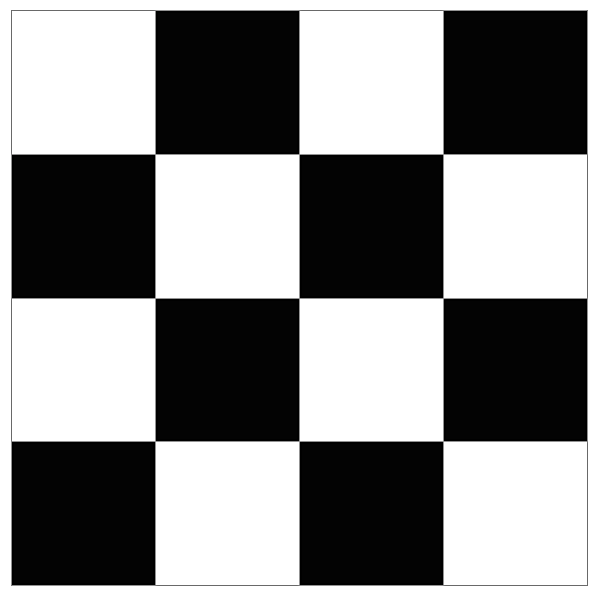
The cellular automata diagrams that Wolfram uses have boxes with thin lines, rather than just a raster image with 1's and 0's represented by borderless boxes. They're particularly appealing because the lines are white between black boxes and black between white boxes, which makes the structures very easy to see. After some digging, I found that, naturally, a Mathematica function to create those box diagrams does exist, and it's called ArrayPlot, with the Mesh option set to True:
In[9]:= ArrayPlot[Table[Mod[i + j, 2], {i, 0, 3}, {j, 0, 3}], Mesh -> True]
Out[9]=

While we could just use ArrayPlot, it' s important when developing software to encapsulate our knowledge as much as possible, so we'll create a function CAGridGraphics (following the way Wolfram named his functions) that encapsulates the knowledge of turning the Mesh option to True. If later we decide there's a better representation, we can just update CAMeshGraphics, rather than hunting down every use of ArrayPlot. This function gives us this:
In[10]:= CAMeshGraphics[matrix_List] :=
ArrayPlot[matrix, Mesh -> True, ImageSize -> Large]
In[11]:= CAMeshGraphics[{CenterList[10], CenterList[10]}]
Out[11]=

Now, Wolfram has these great diagrams to help visualize cellular automata rules which show the neighbors up top and the output value at bottom, with a space between them. The GraphicsGrid does what we want here, except it by its nature resizes all the graphics to fill each available box. I'm sure there's a clever way to do this, but I don't know Mathematica well enough to find it, so I'm going to go back on what I just said earlier, break out the options on ArrayPlot, and tell the boxes to be the size I want:
In[20]:= CATransitionGraphics[rule_List] :=
GraphicsGrid[
Transpose[{Map[
ArrayPlot[{#}, Mesh -> True, ImageSize -> {20 Length[#], 20}] &, rule]}]]
That works reasonably well; here' s an example rule, where three live neighbors in a row kills the center cell :
In[21]:= CATransitionGraphics[{{1, 1, 1}, {0}}]
Out[21]=

Now we need the pattern of digits that Wolfram uses to represent his neighbor patterns. Looking at the diagrams and sfter some digging in the code, it seems like these digits are simply listed in reverse counting order - that is, for 3 cells, we count down from 2^3 - 1 to 0, represented as binary digits.
In[22]:= CANeighborPattern[num_Integer] :=
Table[IntegerDigits[i, 2, num], {i, 2^num - 1, 0, -1}]
In[23]:= CANeighborPattern[3]
Out[23]= {{1, 1, 1}, {1, 1, 0}, {1, 0, 1}, {1, 0, 0}, {0, 1, 1}, {0, 1, 0}, {0, 0,
1}, {0, 0, 0}}
Stay with me - that only gets us the first row of the CATransitionGraphics; to get the next row, we need to apply a rule to that pattern and take the center cell:
In[24]:= CARuleCenterElement[rule_List, pattern_List] :=
CAStep[rule, pattern][[Floor[Length[pattern]/2]]]
In[25]:= CARuleCenterElement[ElementaryRule[30], {0, 1, 0}]
Out[25]= 1
With all this, we can now generate the pattern of 1' s and 0' s that represent the transitions for a single rule:
In[26]:= CARulePattern[rule_List] :=
Map[{#, {CARuleCenterElement[rule, #]}} &, CANeighborPattern[3]]
In[27]:= CARulePattern[ElementaryRule[30]]
Out[27]= {{{1, 1, 1}, {0}}, {{1, 1, 0}, {1}}, {{1, 0, 1}, {0}}, {{1, 0, 0}, {1}}, {{0,
1, 1}, {0}}, {{0, 1, 0}, {1}}, {{0, 0, 1}, {1}}, {{0, 0, 0}, {0}}}
Now we can turn it into graphics, putting it into another GraphicsGrid, this time with a Frame.
In[28]:= CARuleGraphics[rule_List] :=
GraphicsGrid[{Map[CATransitionGraphics[#] &, CARulePattern[rule]]},
Frame -> All]
In[29]:= CARuleGraphics[ElementaryRule[30]]
Out[29]=

At last! We' ve got the beautiful transition diagrams that Wolfram has in his book. And we want to apply it to a row with a single cell:
In[30]:= CAMeshGraphics[{CenterList[43]}]
Out[30]=

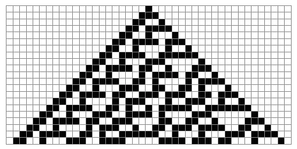
What does that look like? Well, we once again take our CAEvolveList function from before, but rather than formatting it with Raster, we format it with our CAMeshGraphics:
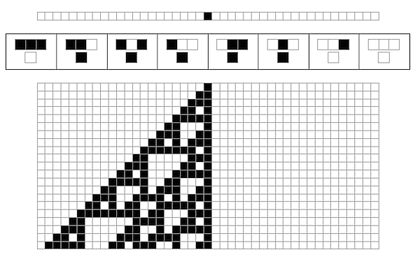
In[31]:= CAMeshGraphics[CAEvolveList[ElementaryRule[30], CenterList[43], 20]]
Out[31]=

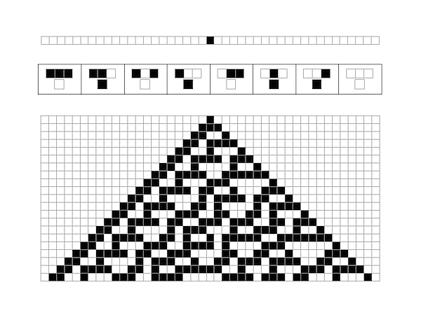
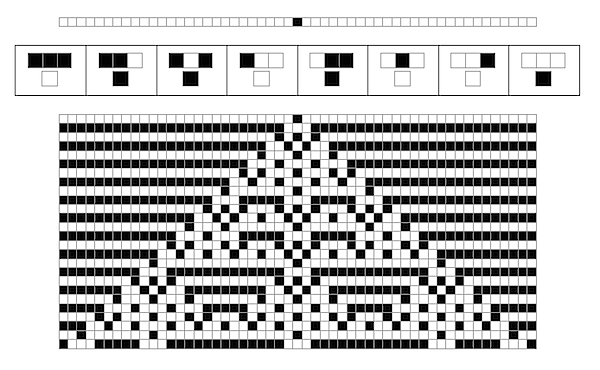
And now we' ve got all the parts of the graphics which appear in the initial diagram of this page. Just to work it out a bit further, let’s write a single function to put all the graphics together, and try it out on rule 110, the rule which Wolfram discovered could effectively simulate any possible program, making it effectively a universal computer:
In[22]:= CAApplicationGraphics[rule_Integer, size_Integer] := Column[
{CAMeshGraphics[{CenterList[size]}],
CARuleGraphics[ElementaryRule[rule]],
CAMeshGraphics[
CAEvolveList[ElementaryRule[rule], CenterList[size],
Floor[size/2] - 1]]},
Center]
In[23]:= CAApplicationGraphics[110, 43]
Out[23]=

It doesn' t come out quite the way it did in Photoshop, but we' re getting close. Further learning of the rules of Mathematica graphics will probably help me, but that's neither here nor there. We've got a set of tools for displaying diagrams, which we can craft into what we need.
Which happens to be a non-standard number system unfolding itself into hyperbolic space, God help me.
Wish me luck.
-the Centaur
P.S. While I' m going to do a standard blogpost on this, I' m also going to try creating a Mathematica Computable Document Format (.cdf) for your perusal. Wish me luck again - it's my first one of these things.
P.P.S. I think it' s worthwhile to point out that while the tools I just built help visualize the application of a rule in the small …
In[24]:= CAApplicationGraphics[105, 53]
Out[24]=

... the tools Wolfram built help visualize rules in the very, very large:
In[25]:= Show[CAGraphics[CAEvolveList[ElementaryRule[105], CenterList[10003], 5000]]]
Out[25]=

That's 10,000 times bigger - 100 times bigger in each direction - and Mathematica executes and displays it flawlessly.


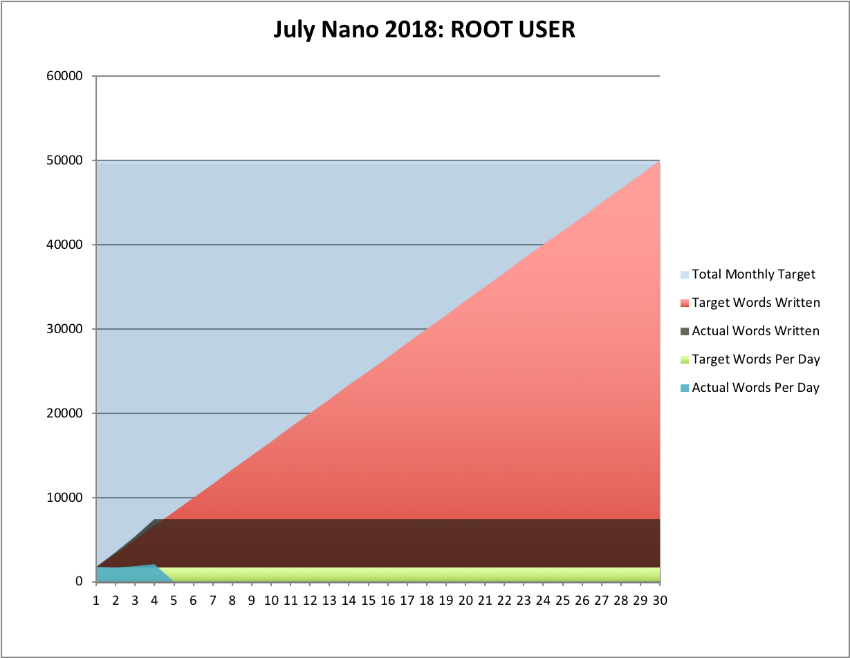 Well, the Nano climb is starting off great, for a switch! Fourth of July, and I'm already 800 words ahead of what my goal is for this time of the month.
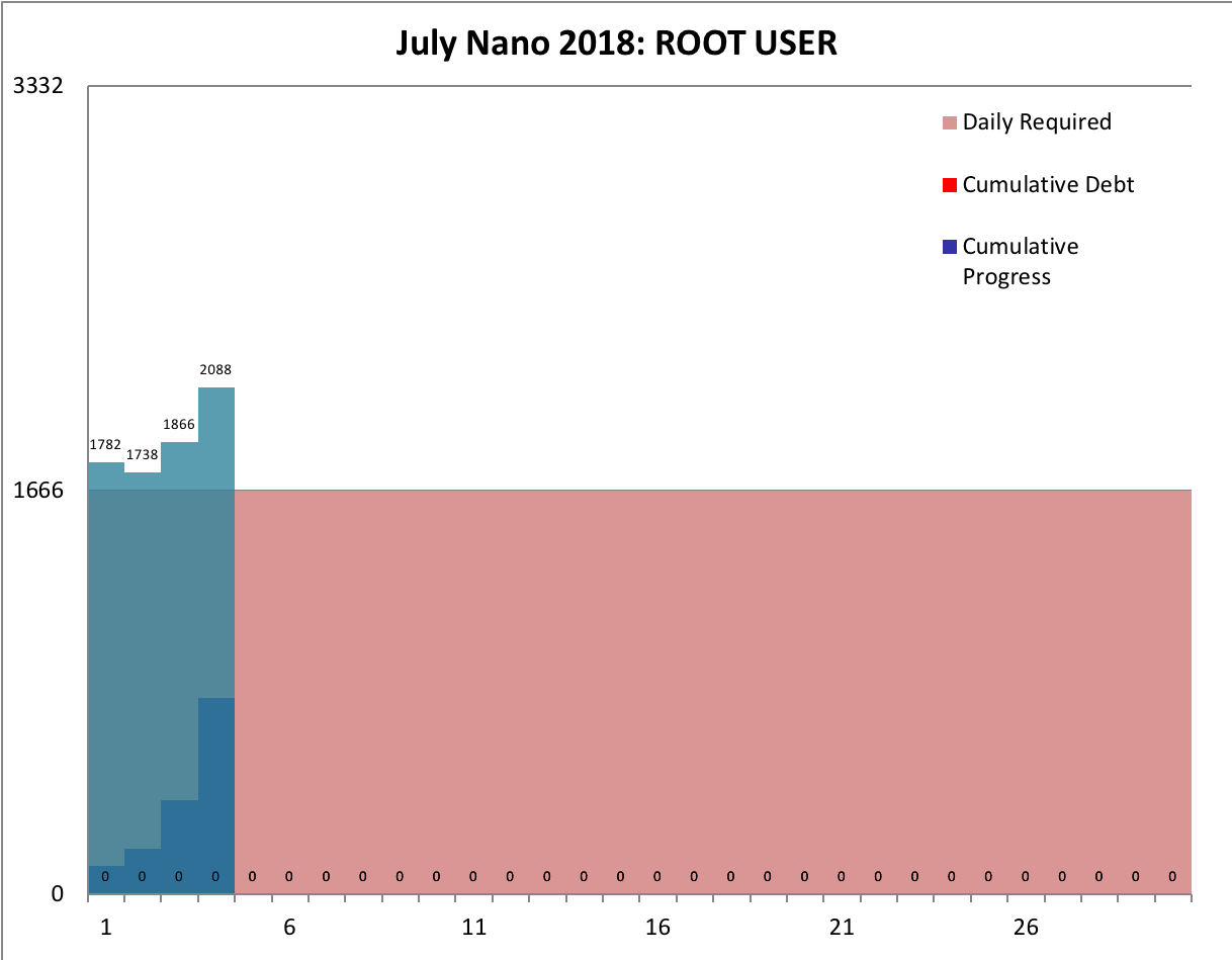 Not bad, but then, I am on vacation. :-) An excerpt:
 Well, so insanely busy, I haven't posted in a while. But not for want of working on things that I want to post about! Most pressingly, my Camp Nano project for the July Camp of 2018, and what I hope is the last major chunk of the third book in the Cinnamon Frost series ...
  Hail, fellow adventurers! And now you know why you haven't heard from me for a while: I was heads down finishing my wordcount for Camp Nanowrimo! And this is a very special one, because it marks the twentieth time I have won a National Novel Writing Month style challenge to write 50,000 words of a novel in a month! Woohoo! When I started, I never thought I'd finish this many!
 This was a difficult month for it. Sure, I just finished early, but that final push involved locking me in a downstairs room with my laptop until I finished so I could enjoy the rest of my vacation with my wife. And the push up to this point has been hard: my wife returning from vacation, with me scrambling to finish a spring cleaning gone awry before she got home. A cat being treated for cancer. An organization I'm volunteering with had an emergency that involved multiple meetings over the month. Major shifts and dustups at work. Robots, on the loose, being chased down the corridors. Ok, that last one isn't real. Well, actually, it was, but it was much, much, much more prosaic than it sounds.
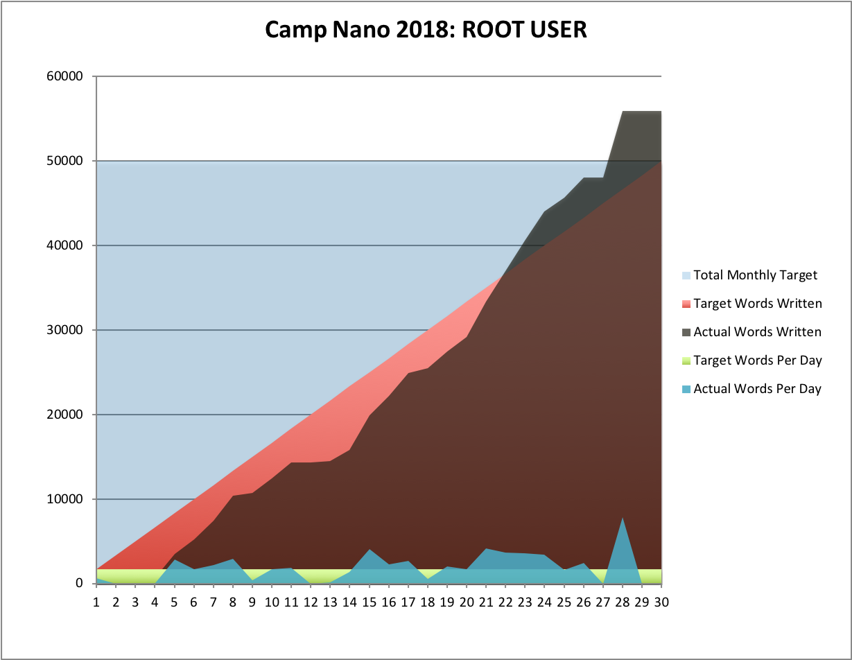
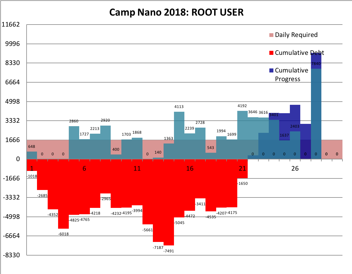 The upshot, seen above, is blood on the water (behind on my wordcount) for most of the month. And with the very last weekend of the month being my long-planned vacation in Monterey with my wife before she flies out on her next business trip, there was a very real danger that I wouldn't make it. But my wife is awesome, and tolerated me taking out this first evening to do a massive push to get all my words done!
 And now, sleep. But first, an excerpt:
 And I'm supposed to tell you that my biographer, Anthony Francis, is working on my third book, ROOT USER, for
  When I was a kid (well, a teenager) I'd read puzzle books for pure enjoyment. I'd gotten started with Martin Gardner's mathematical recreation books, but the ones I really liked were Raymond Smullyan's books of logic puzzles. I'd go to Wendy's on my lunch break at Francis Produce, with a little notepad and a book, and chew my way through a few puzzles. I'll admit I often skipped ahead if they got too hard, but I did my best most of the time.
I read more of these as an adult, moving back to the Martin Gardner books. But sometime, about twenty-five years ago (when I was in the thick of grad school) my reading needs completely overwhelmed my reading ability. I'd always carried huge stacks of books home from the library, never finishing all of them, frequently paying late fees, but there was one book in particular - The Emotions by Nico Frijda - which I finished but never followed up on.
Over the intervening years, I did finish books, but read most of them scattershot, picking up what I needed for my creative writing or scientific research. Eventually I started using the tiny little notetabs you see in some books to mark the stuff that I'd written, a "levels of processing" trick to ensure that I was mindfully reading what I wrote.
A few years ago, I admitted that wasn't enough, and consciously began trying to read ahead of what I needed to for work. I chewed through C++ manuals and planning books and was always rewarded a few months later when I'd already read what I needed to to solve my problems. I began focusing on fewer books in depth, finishing more books than I had in years.
Even that wasn't enough, and I began - at last - the re-reading project I'd hoped to do with The Emotions. Recently I did that with Dedekind's Essays on the Theory of Numbers, but now I'm doing it with the Deep Learning. But some of that math is frickin' beyond where I am now, man. Maybe one day I'll get it, but sometimes I've spent weeks tackling a problem I just couldn't get.
Enter puzzles. As it turns out, it's really useful for a scientist to also be a science fiction writer who writes stories about a teenaged mathematical genius! I've had to simulate Cinnamon Frost's staggering intellect for the purpose of writing the Dakota Frost stories, but the further I go, the more I want her to be doing real math. How did I get into math? Puzzles!
So I gave her puzzles. And I decided to return to my old puzzle books, some of the ones I got later but never fully finished, and to give them the deep reading treatment. It's going much slower than I like - I find myself falling victim to the "rule of threes" (you can do a third of what you want to do, often in three times as much time as you expect) - but then I noticed something interesting.
Some of Smullyan's books in particular are thinly disguised math books. In some parts, they're even the same math I have to tackle in my own work. But unlike the other books, these problems are designed to be solved, rather than a reflection of some chunk of reality which may be stubborn; and unlike the other books, these have solutions along with each problem.
So, I've been solving puzzles ... with careful note of how I have been failing to solve puzzles. I've hinted at this before, but understanding how you, personally, usually fail is a powerful technique for debugging your own stuck points. I get sloppy, I drop terms from equations, I misunderstand conditions, I overcomplicate solutions, I grind against problems where I should ask for help, I rabbithole on analytical exploration, and I always underestimate the time it will take for me to make the most basic progress.
Know your weaknesses. Then you can work those weak mental muscles, or work around them to build complementary strengths - the way Richard Feynman would always check over an equation when he was done, looking for those places where he had flipped a sign.
Back to work!
-the Centaur
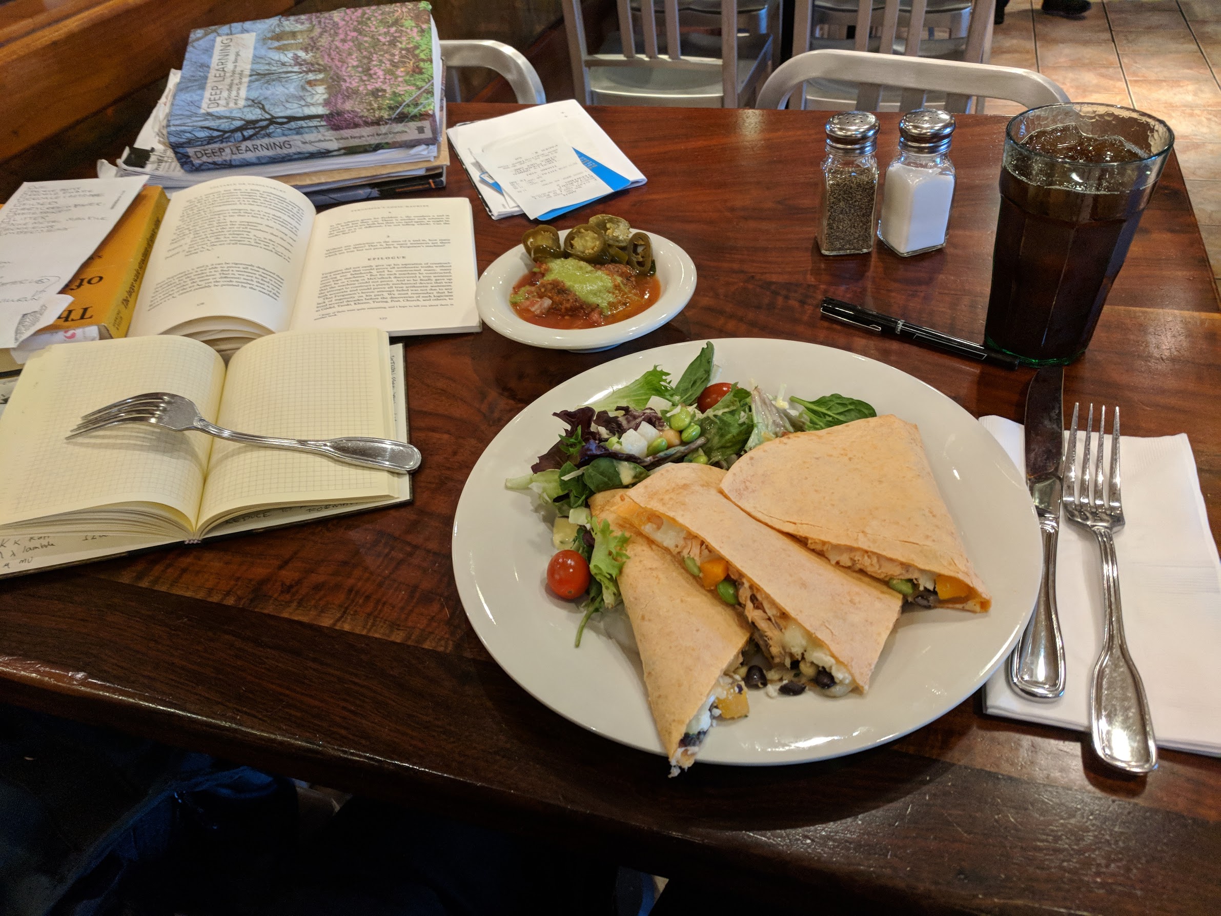
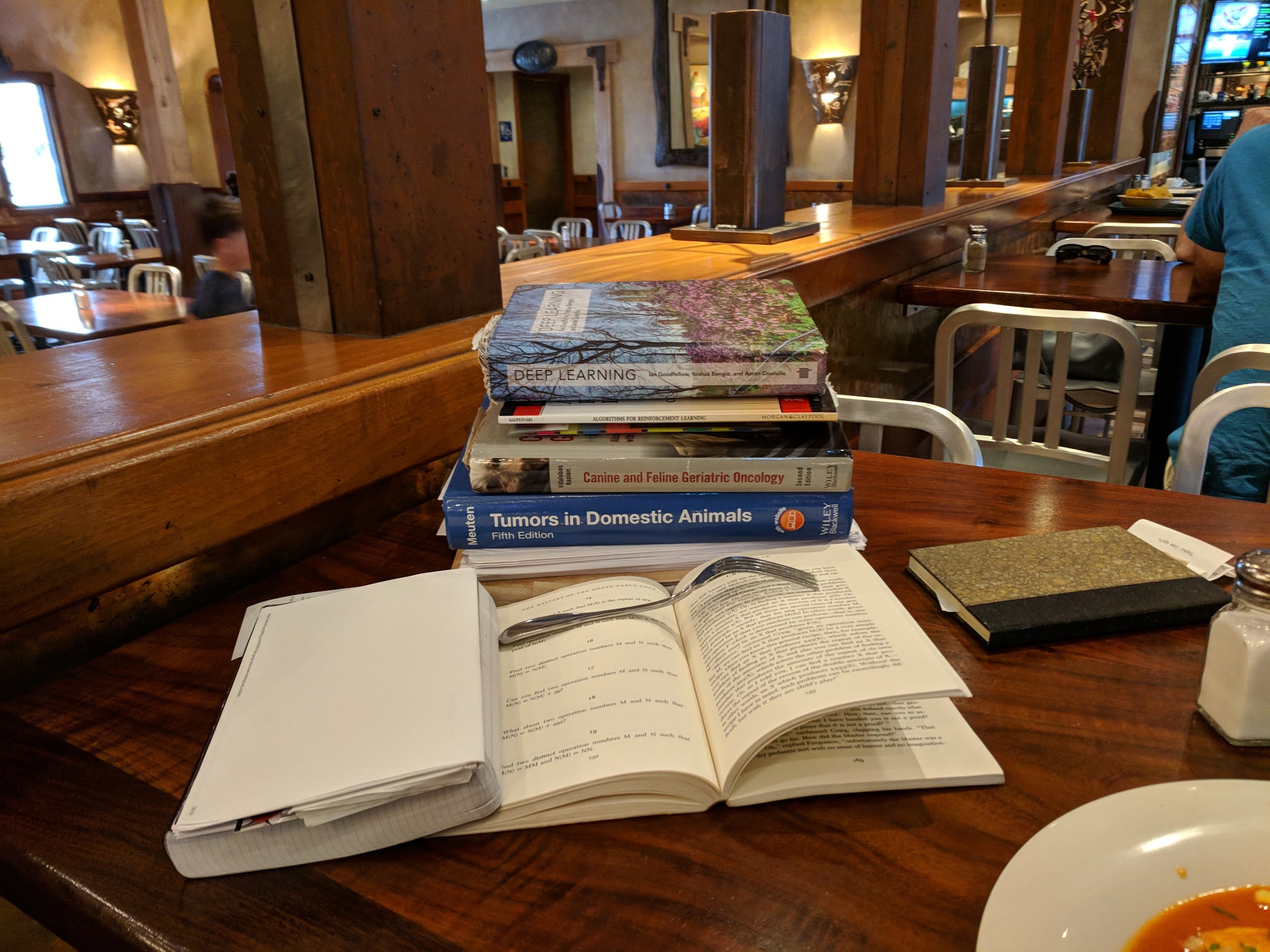
Pictured: my "stack" at a typical lunch. I'll usually get to one out of three of the things I bring for myself to do. Never can predict which one though.
 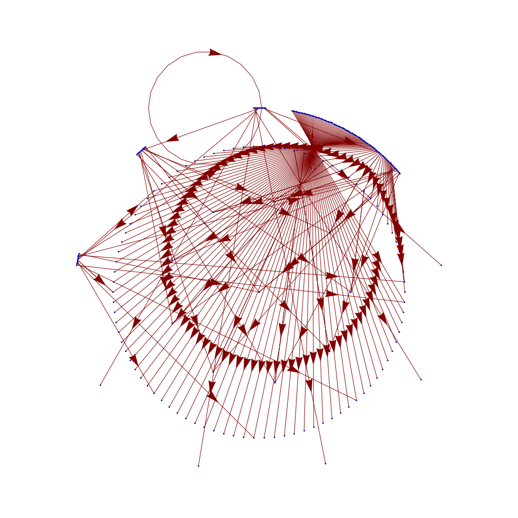 I had way too much data to exploit, so I started to think about culling it out, using the length of the "mumbers" to cut off all the items too big to care about. That led to the key missing insight: my method of mapping mumbers mapped the first digit of each item to the same position - that is, 9, 90, 900, 9000 all had the same angle, just further out. This distance was already a logarithm of the number, but once I dropped my resistance to taking the logarithm twice...
 ... then I could create a transition plot function which worked for almost any mumber in the sets of mumbers I was playing with ...
 Then I could easily visualize the small set of transitions - "mumbers" with 3 digits - that yielded the graph above; for reference these are:
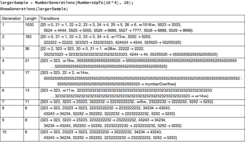
 The actual samples I wanted to play with were larger, like this up to 4 digits:
 This yields a still visible graph:
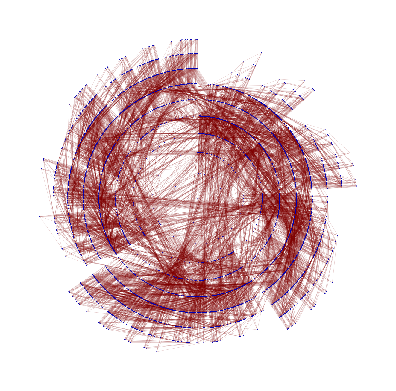
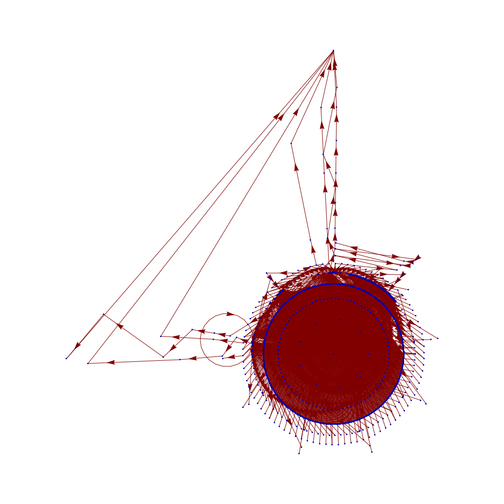 And this, while it doesn't let me visualize the whole space that I wanted, does provide the insight I wanted. The "mumbers" up to 10000 do indeed "produce" most of the space of the smaller "mumbers" (not surprising, as the "mumber" rule 2XYZ produces XYZ, and 52XY produces XYXY ... meaning most numbers in the first 10,000 will be produced by one in that first set). But this shows that sequences of 52 rule transitions on the left produce a few very, very large mumbers - probably because 552552 produces 552552552552 which produces 552552552552552552552552552552552552 which quickly zooms away to the "mumberOverflow" value at the top of my chart.
And now the next lesson: finishing up this insight, which more or less closes out what I wanted to explore here, took 45 minutes. I had 15 allotted to do various computer tasks before leaving Aqui, and I'm already 30 minutes over that ... which suggests again that you be careful going down rabbit holes; unlike leprechaun trails, there isn't likely to be a pot of gold down there, and who knows how far down it can go?
-the Centaur
P.S. I am not suggesting this time spent was not worthwhile; I'm just trying to understand the option cost of various different problem solving strategies so I can become more efficient.
 SO! There I was, trying to solve the mysteries of the universe, learn about deep learning, and teach myself enough puzzle logic to create credible puzzles for the Cinnamon Frost books, and I find myself debugging the fine details of a visualization system I've developed in Mathematica to analyze the distribution of problems in an odd middle chapter of Raymond Smullyan's
  I meant well! Really I did. I was going to write a post about how finding a solution is just a little bit harder than you normally think, and how insight sometimes comes after letting things sit.
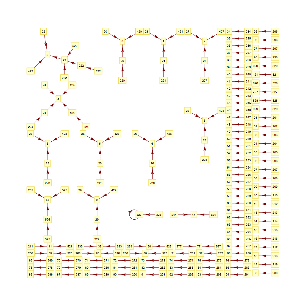 But the tools I was creating didn't do what I wanted, so I went deeper and deeper down the rabbit hole trying to visualize them.
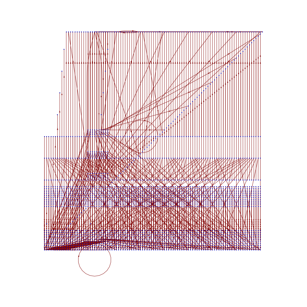 The short answer seems to be that there's no "there" there and that further pursuit of this sub-problem will take me further and further away from the real problem: writing great puzzles!
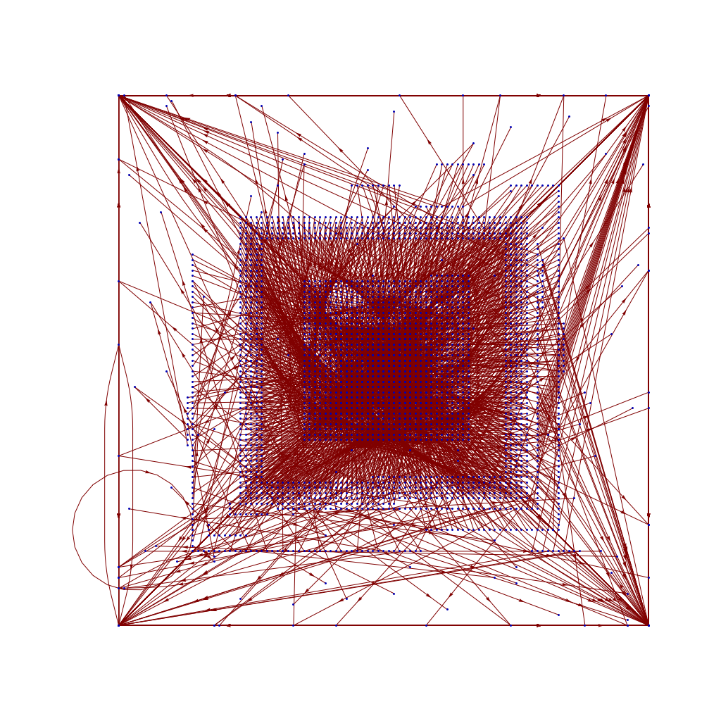 I learned a lot - about numbers, about how things could combinatorially explode, about
 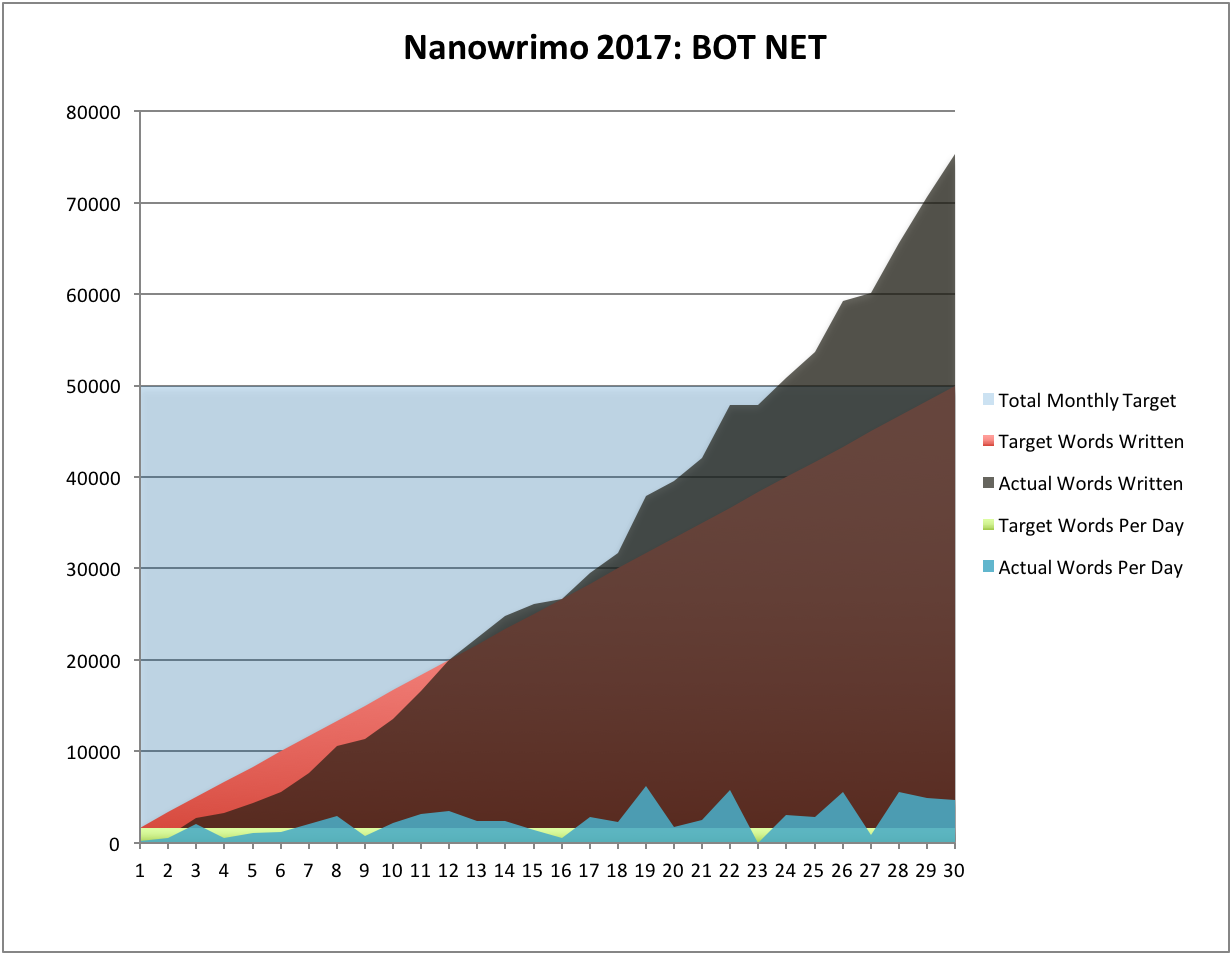 This somehow all magically happened because I never lost my momentum after the Night of Writing Dangerously, oh, and because this is Cinnamon Frost, and she's awesome!
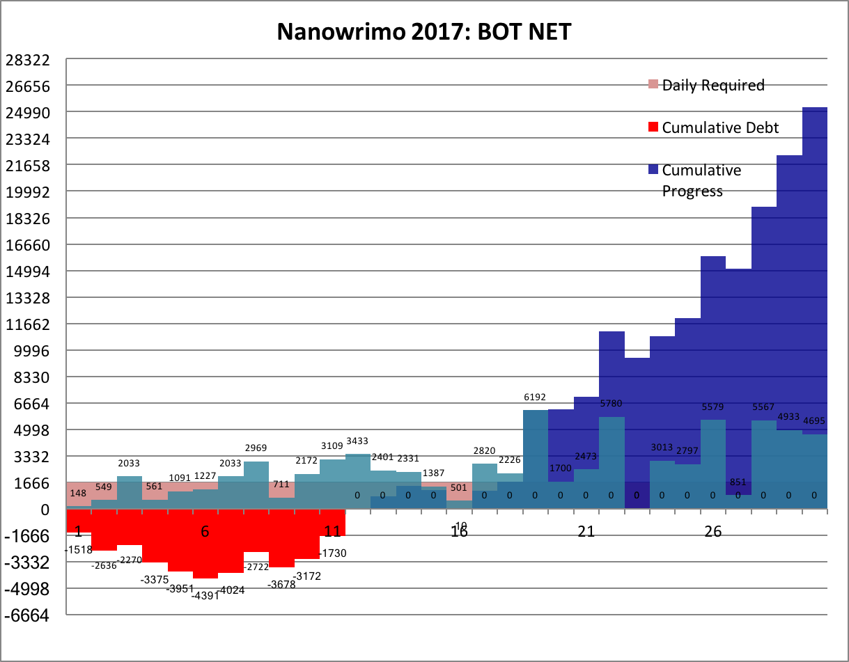 This is the most I've ever written in Nano, by a long shot - almost 10,000 words more. Not quite, and I'm not super motivated to make it exactly 10,000 words more. If I think of more words tonight, eh maybe.
 Oh yes, the traditional excerpt:
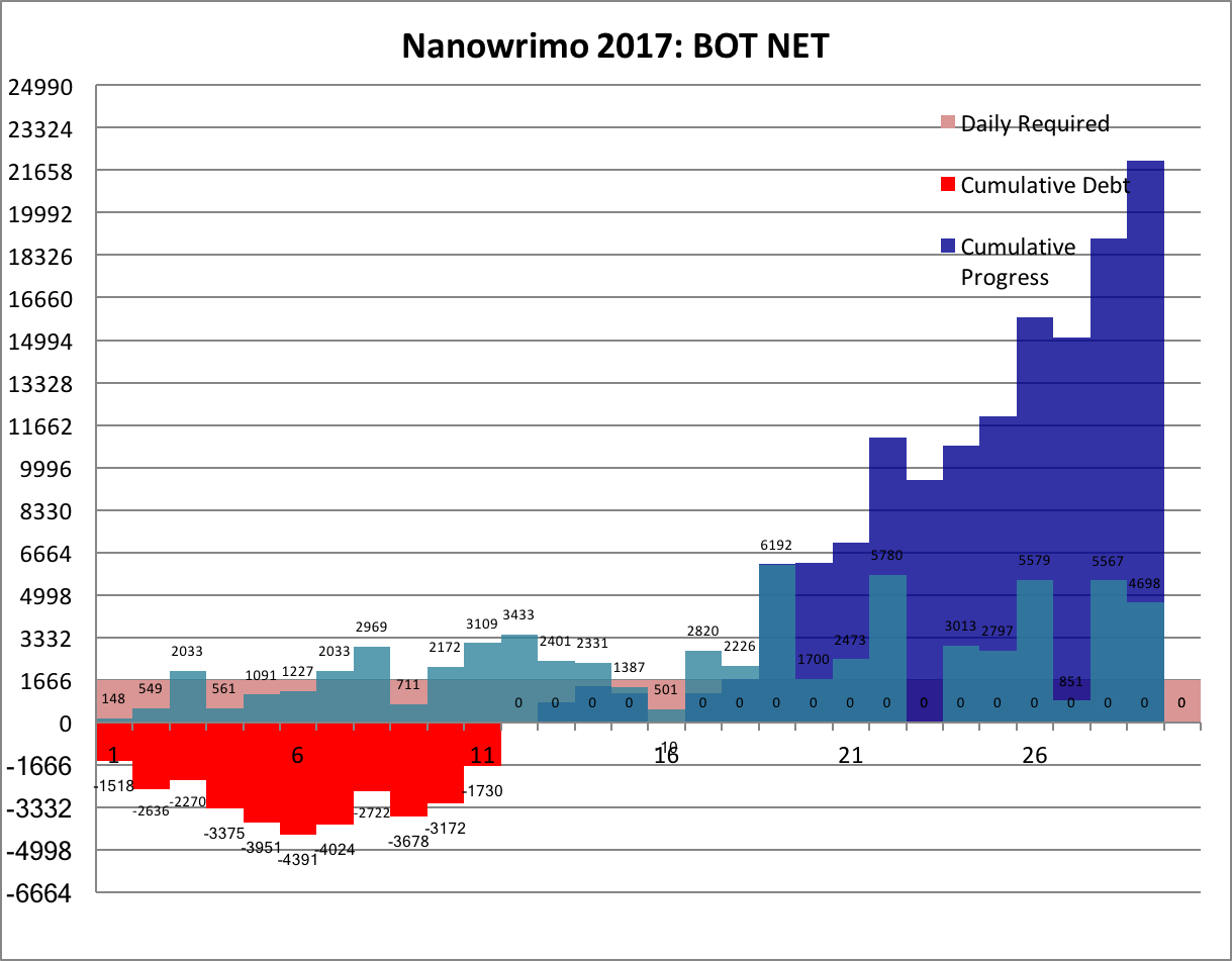 I won't just beat my best record ever (which I already have) ...
 ... I'll hit the somewhat ludicrous amount of 75,000 words in a month, beyond the 70,000 I've already hit.
 4,648 words to hit that goal ... less than I did yesterday or even today. Let's get cracking.
-the Centaur
 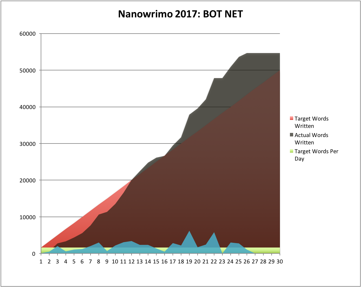 ~2900 words a day, not counting today ...
 I will beat my all time Nanowrimo record of 65,995 words:
 Sounds like a worthier goal than spending the same words responding to everyone who's wrong on the Internet.
Onward!
-the Centaur
  This year, I was working on
 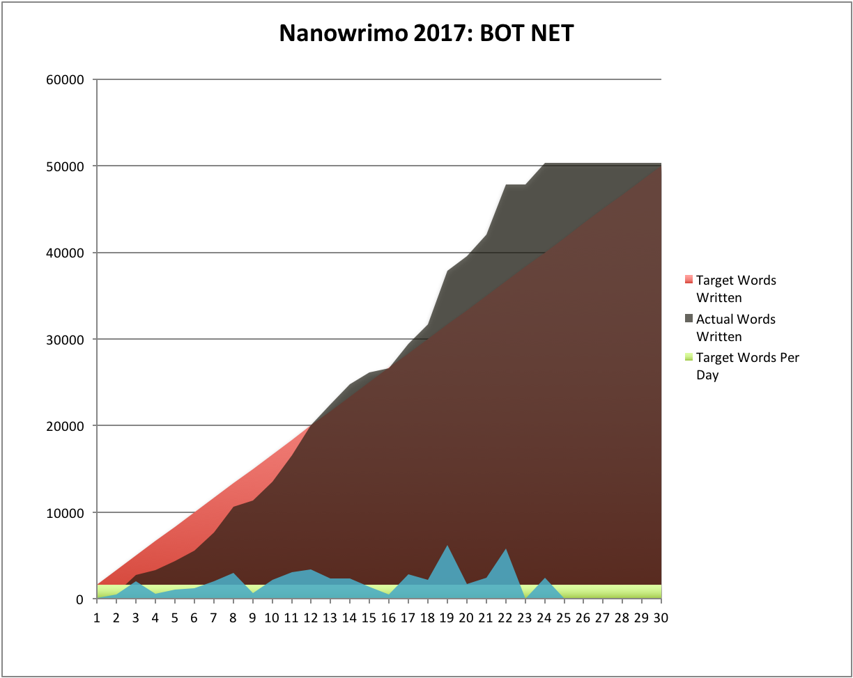 This year, the combination of participating in the
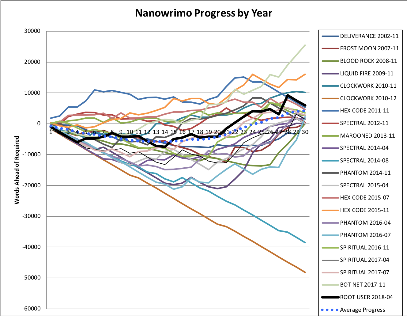
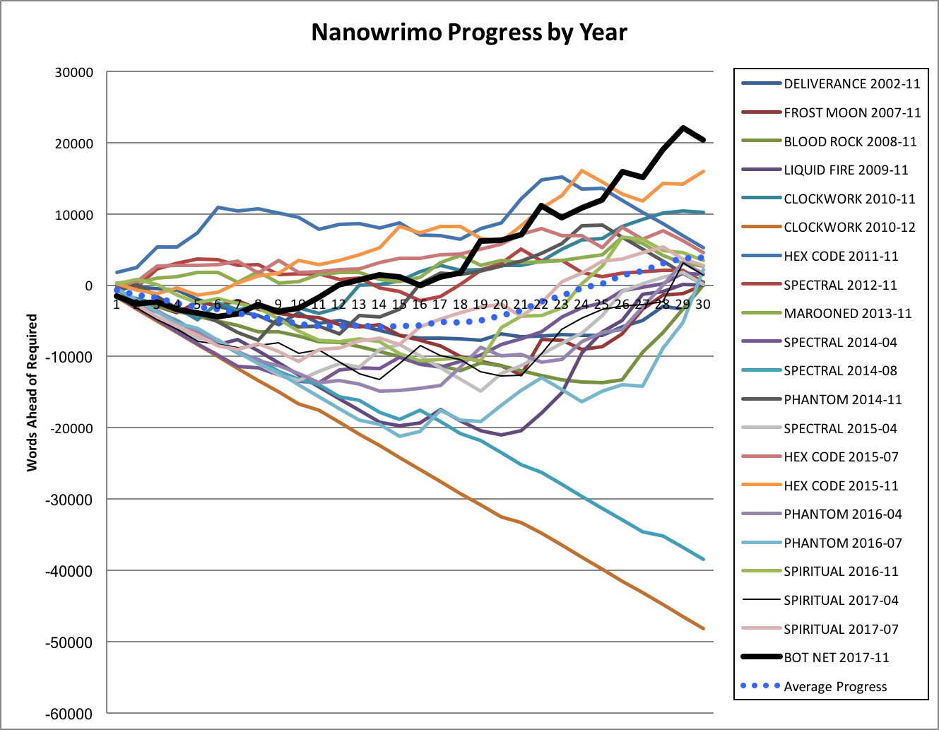
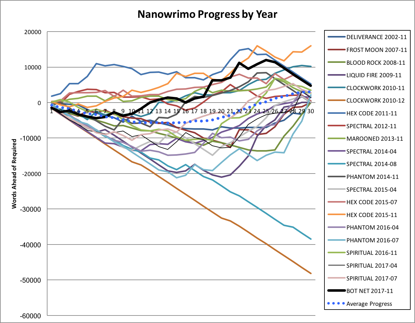
 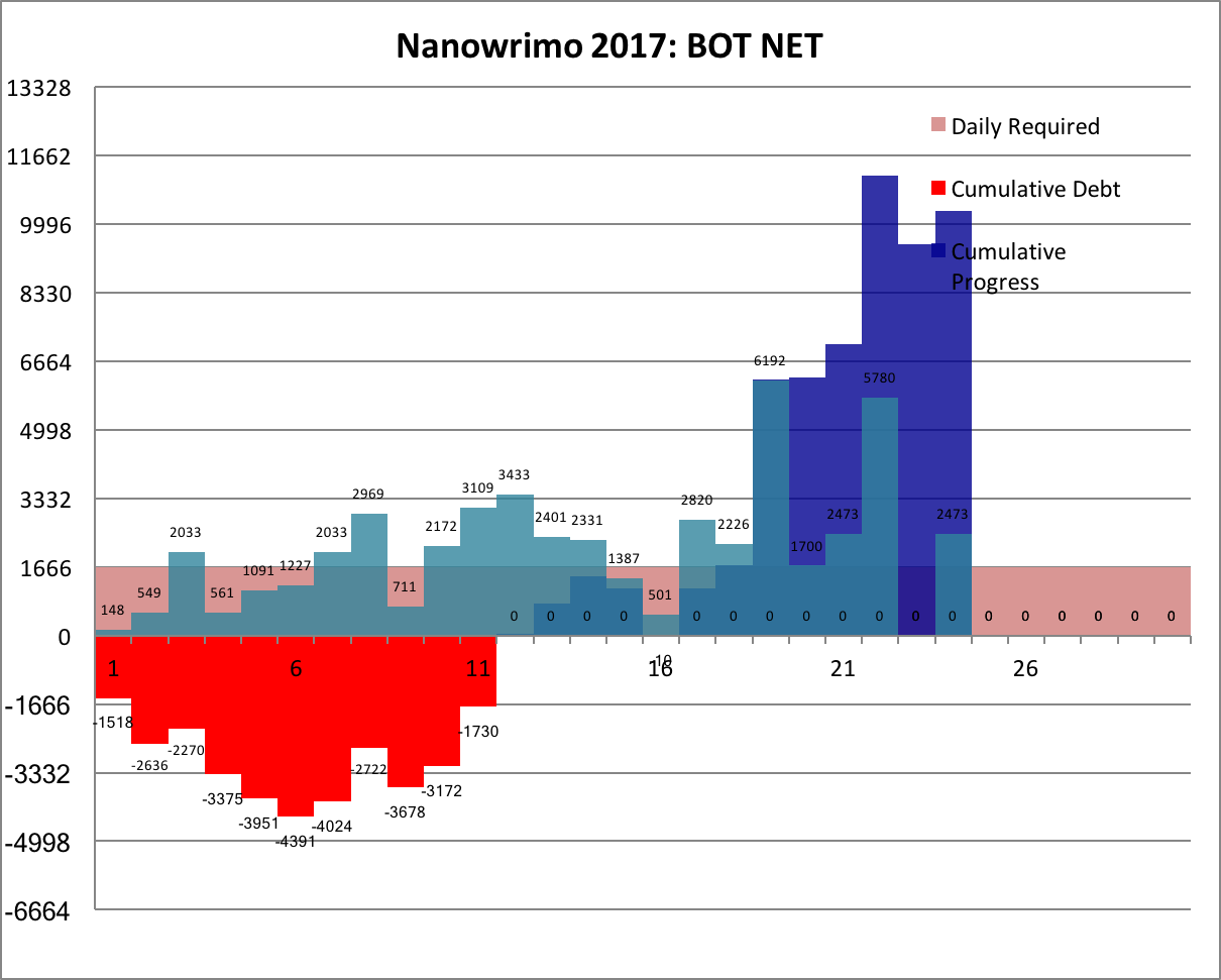 Interesting, the hole at Thanksgiving. I wonder if that's true every year? That's not something you can readily see when you look at the yearly charts since it moves (stay tuned, these charts are going to come back later):
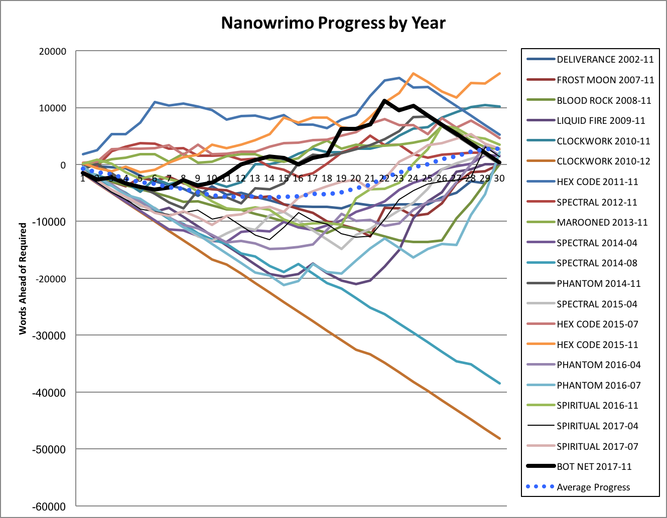 There was a time when almost every post about Nanowrimo I'd include an excerpt. Frankly, that's gotten harder to do as I've switched from doing Nano once per year to three times per year; the Nano material has become more inchoate as I blaze new paths out into story space, requiring more work to turn it into final material. But, occasionally, I can indeed include some material that gives you a flavor ...
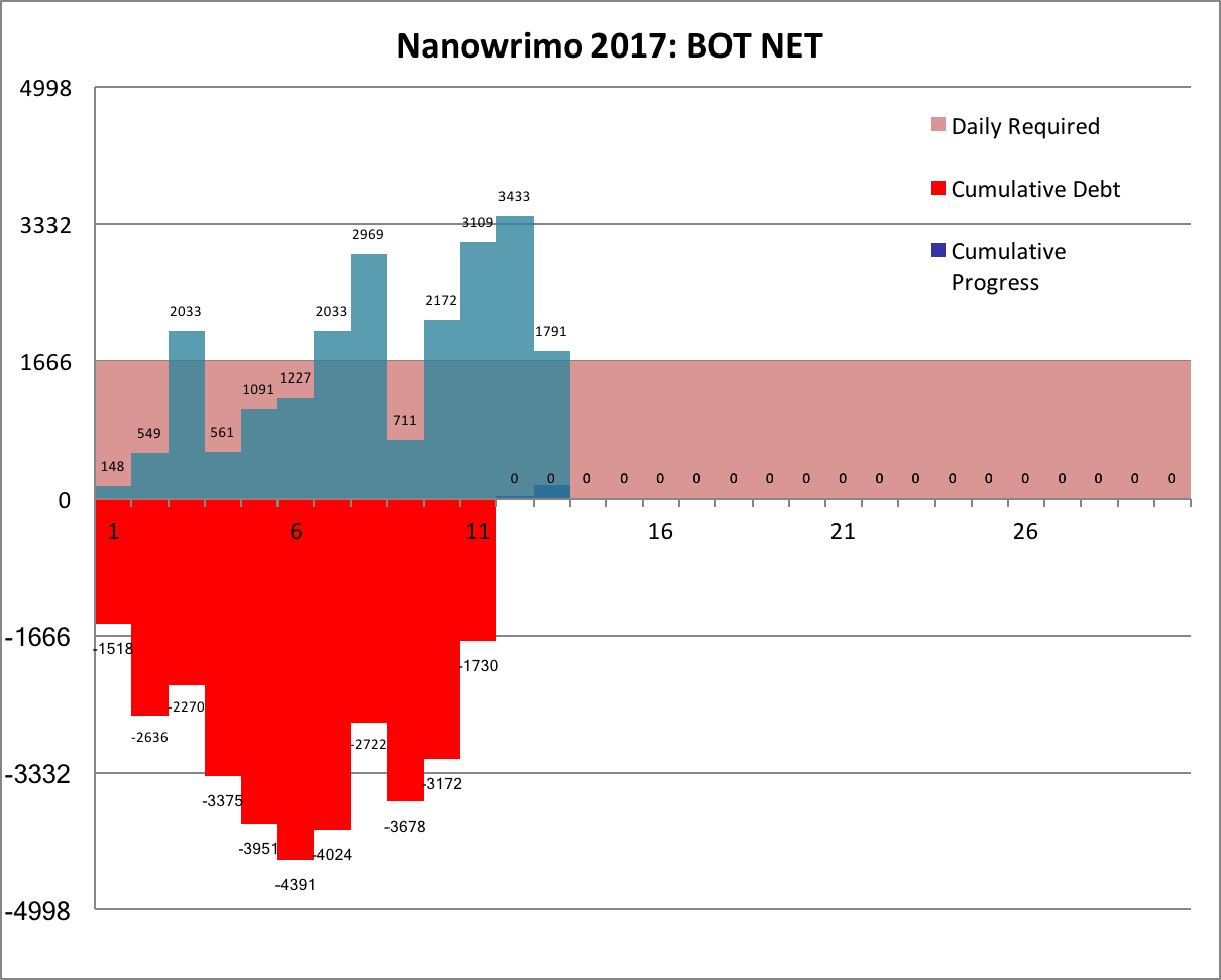 Winning at Nano always feels like climbing a hill, but for me in particular it almost always feels like I start out sliding back down, Sisyphus-like, as I struggle to get a handle on the story.
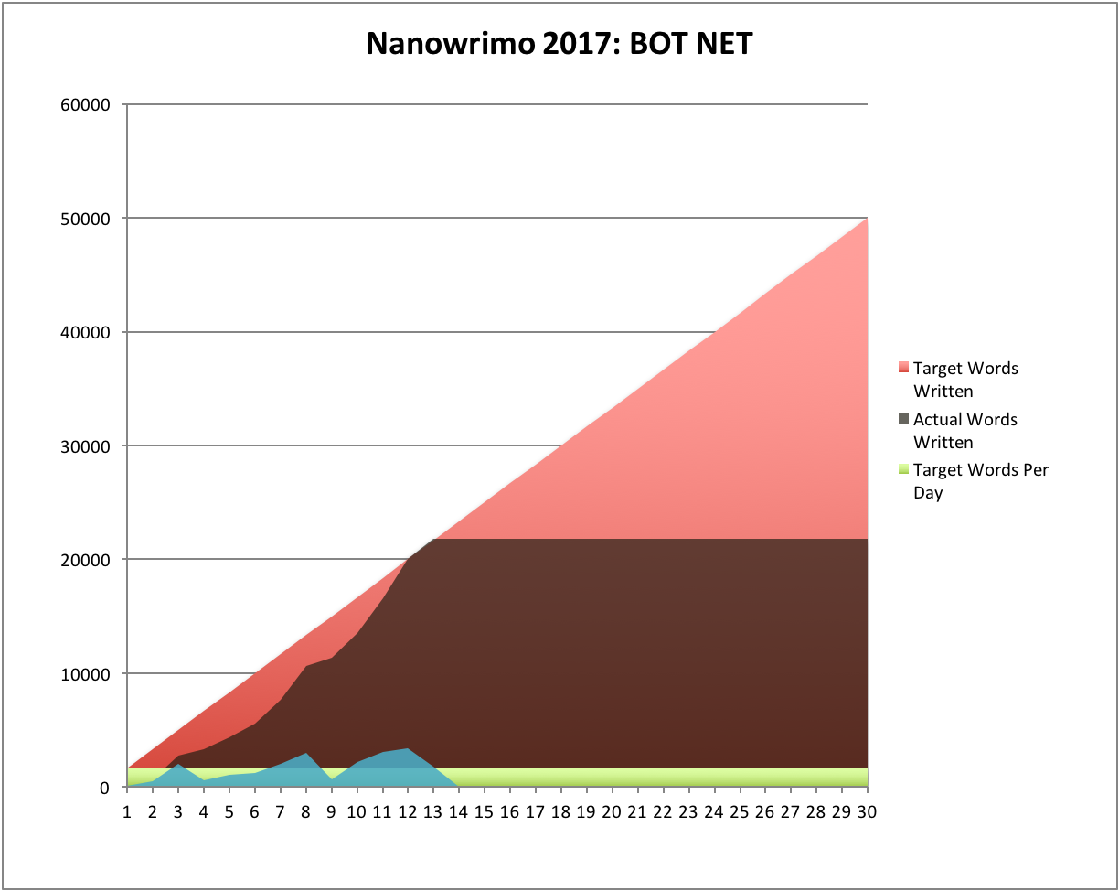 But then there comes that magic point where I need to write 1,666 words in a day and I. Got. Nothing. Then I'm forced to be creative, and the real fun stuff happens, an event I call "going off the rails". Hey, let's try to embed a tweet!
 I'm one more thing too: 200,000 words into the Cinnamon Frost trilogy.
 There are 3 published Dakota Frost novels:
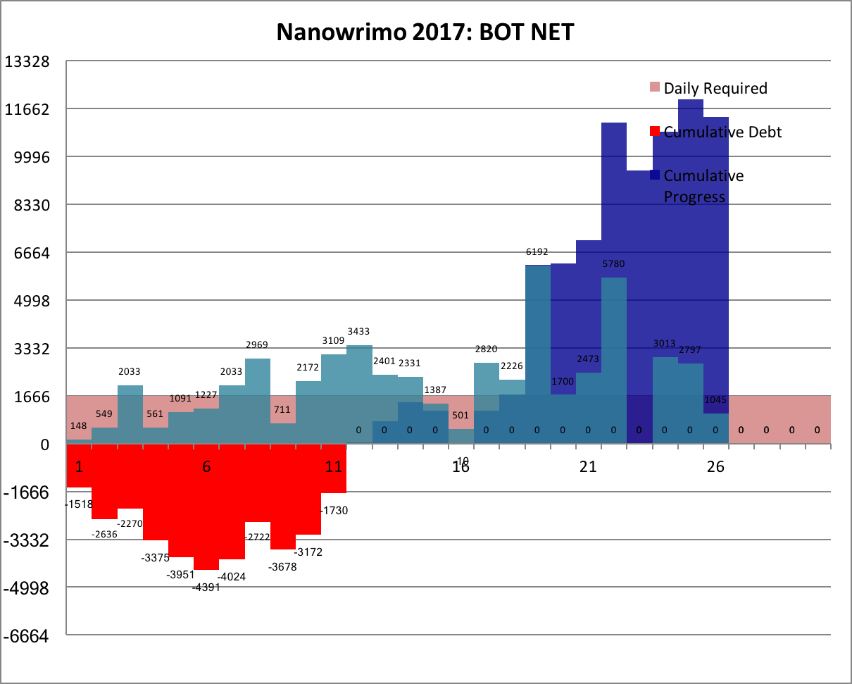
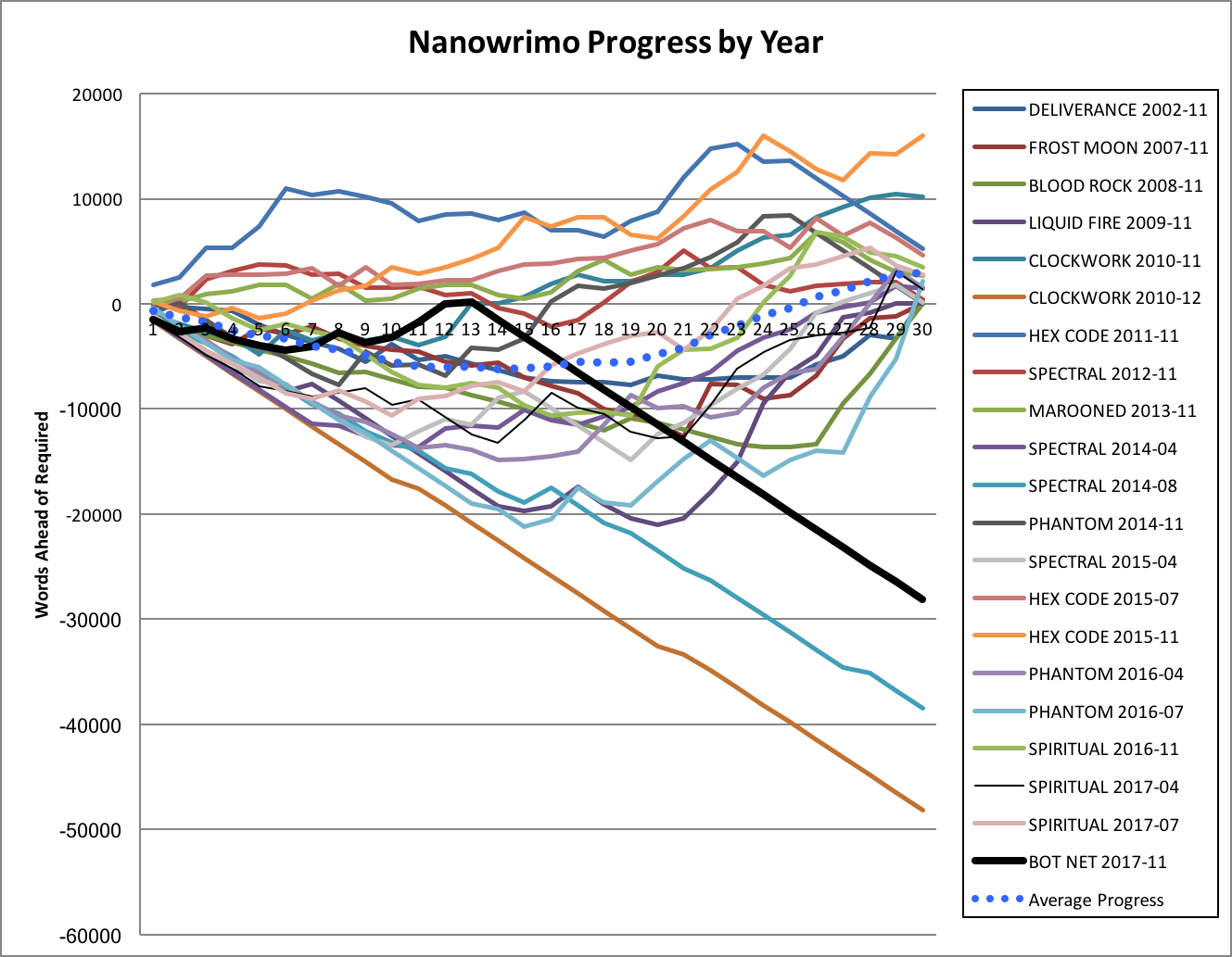
 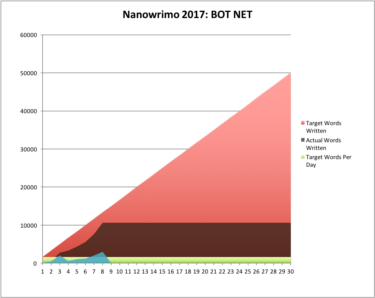 The bad news: I need to be at 13,333 words by today!
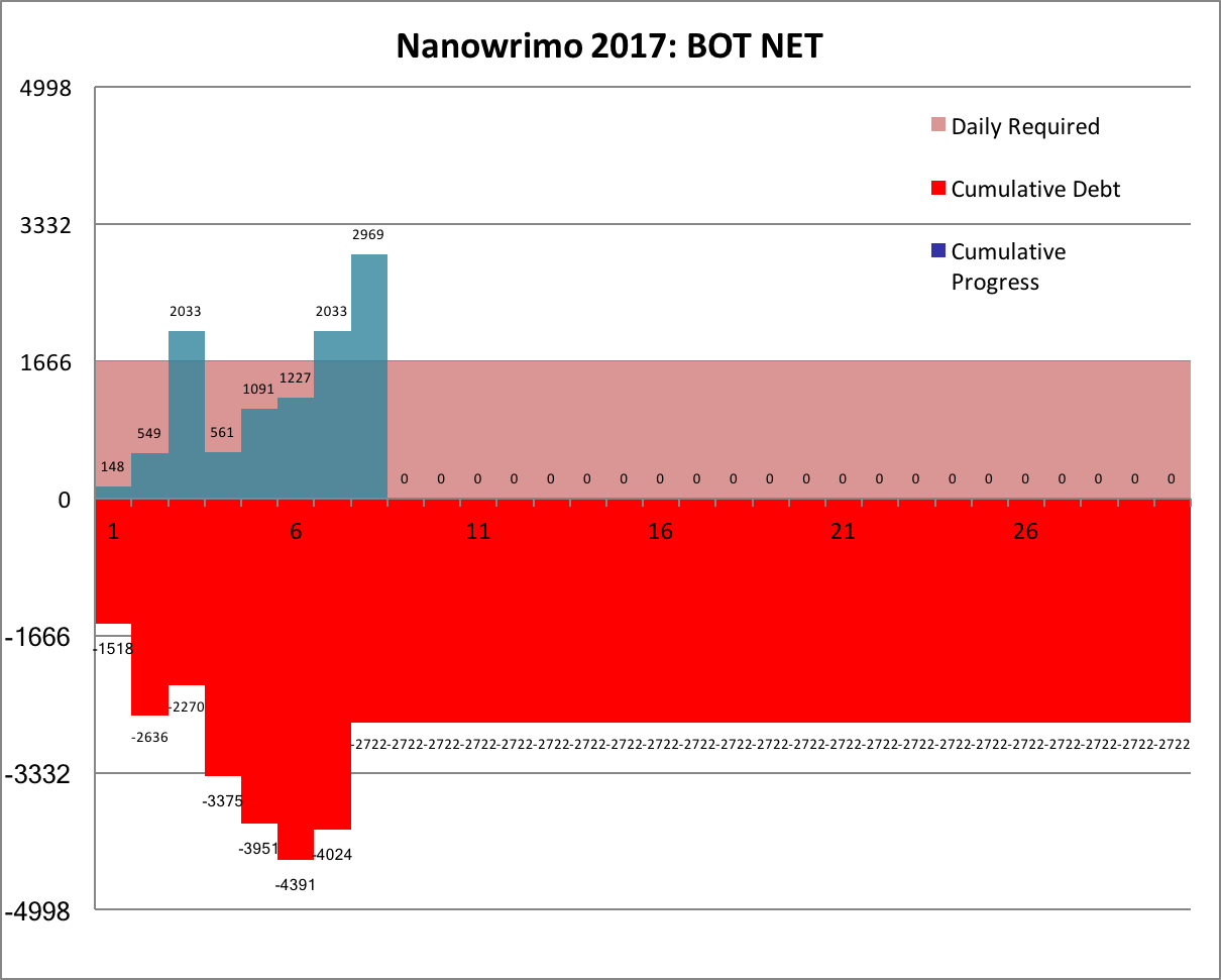 The good-bad news is, normally I'm closer to 4500 words behind at this point of Nano, so I am ahead of where I am normally behind:
 What can I. say? "Don't get cocky, kid." Back to it ...
-the Centaur
 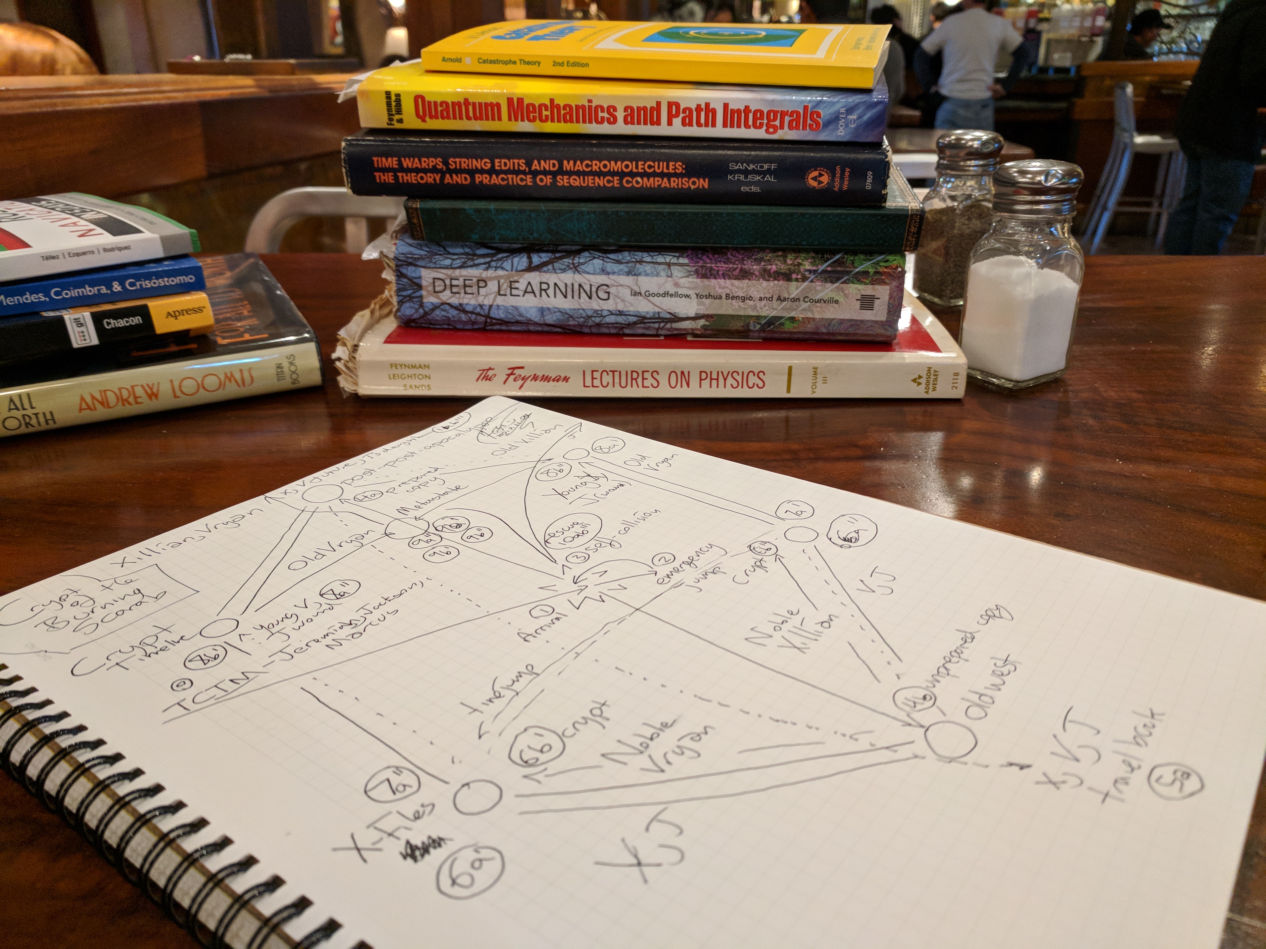 No progress on
  "Okay, so ... um, hi! I'm Cinnamon Frost, and I'm here to tell you that my biographer, Anthony Francis, is busy as fuck writing
 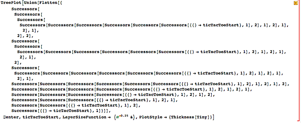 NOT the most elegant Mathematica, but trying to do clever things with NestList was a pain. And my math was creating duplicate transitions, which is why the other graphs were so dense - and the layer size needed to be tweaked a bit to show both the starting and ending states more clearly. But, after some cleanup, it worked, after a bit of churning (click the image for a larger size):
